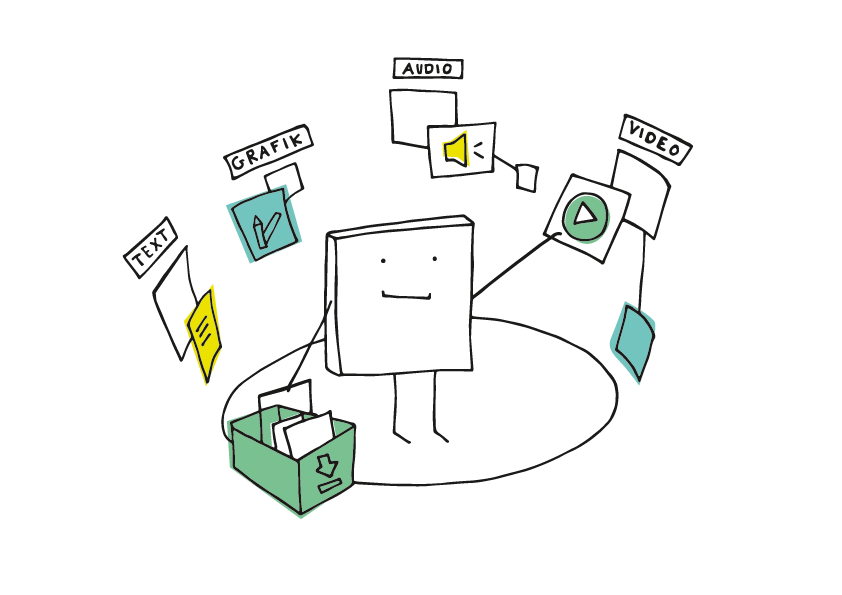
Any research is based on data. Data can come in various forms. Depending on how you approach it data can be classified according to various schemes.
Data comes in various formats. Cartoon by Manfred Steger CC by SA.
Analysing each type of data requires a different framework and methodology. Also, the methods for collecting each type of data may be different.
The word data is a plural form of Latin word datum which means literally ‘something given’, neuter past participle of dare ‘give’. Though plural, in modern use it is treated as mass noun which takes a singular verb. For example, sentences such as “data was collected via online questionnaire” are now widely accepted.
But let us ask ourselves these fundamental questions: What is data? and How do we get data?
2.1 What is data?
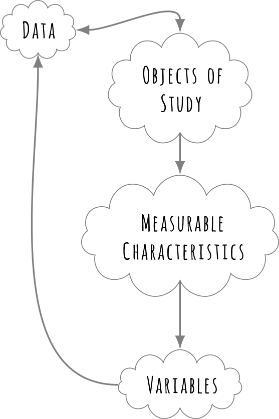
At a very basic level data is information about the objects that we want to understand. Depending on what the field of study is the object of study may be a single cell, a single student, a group of students, a classroom, a school, a district, a state, a country, a document, an interview, a group discussion or the entire universe as in the case of cosmology!
Humans have been collecting and storing data in various forms since antiquity. The data stored in physical format such as inscriptions, papyrus rolls, cuneiform tablets or even oral traditions allowed knowledge to be passed over generations. In our present computer driven world, data is usually stored in a digital format.
When we have an “object of interest” we select some features of this object and try to measure them. These “features” can be anything that is “measurable”. For example, it maybe “handedness” in a classroom of students, or their scores on some exam, or their heights. Thus each object of interest can give us several measurements. These measurements are termed as variables.
Data and variables from objects of interest.
2.2 Types of Variables
Traditionally, depending on their we classify two types of variables in educational research , namely the independent and the dependent variables.
The Independent Variable (sometimes called the predictor or explanatory variable) acts as the “cause” or input in our study. It is the condition or characteristic that the researcher manipulates or observes to see its effect. In contrast, the Dependent Variable (often called the outcome or response variable) acts as the “effect” or output. It is the variable that changes in response to the independent variable—in other words, its value depends on the other factor.
For example, in our research about effect of mother tongue instruction. If we ask, “Does the medium of instruction affect reading fluency?”, the Medium of Instruction (Mother Tongue vs. English) is the Independent Variable because it is the condition being compared. The Reading Fluency Score is the Dependent Variable because we expect it to change depending on which medium was used.
Similarly, consider a study on teacher professional development asking, “Does a 3-week training programme improve teacher confidence?” Here, the Training Status (Trained vs. Untrained) is the Independent Variable, while the score on the Confidence Scale is the Dependent Variable. Even in non-experimental studies, such as investigating if parental income predicts drop-out rates, we treat Annual Household Income as the Independent Variable (Predictor) and Dropout Status as the Dependent Variable (Outcome).
2.3 Limitations of Data
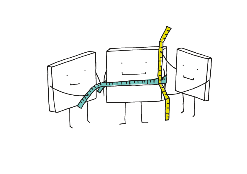
Now this is a fundamental limitation on our ability to get information. For example, we may want to understand thinking processes in the minds of children, but we have only access to what they say and do. This is our data that we can obtain either by experimentation or observation. This data does not tell us directly what we want to know, this is where idea of data analysis comes into picture. We infer from this data about the object of study by analysing this data.
We measure what we can…
The issue is that we can only measure what we can and we build models either mathematical or conceptual based on our analysis of this data. These “models” then help us create a framework for understanding the object of analysis and its variables in relation to each other other contextual variables. This of course is a crude and over simplified description of the actual process.
We measure what we can. Cartoon by Manfred Steger.
What type of measurements are needed to collect your data?
But underlying philosophy that guides such an approach comes from philosophy of science. We assume that by studying and observing the world around us we can collect some data which can be analysed to create models to understand the world. If you ask what is a model, we can perhaps answer:
A postulated structure which approximately could have led to data.
Such models help us think about the world in abstract concepts, and helps us reveal patterns, establish relationships and predict outcomes. But we should be remember, as we have seen in the last chapter, that all models are tentative.
This is particular idea is very well captured by this quote by George Bos
All models are wrong. Some are useful.
What Box means here that we are creating approximate and simplified versions of reality using the data that we have. Thus we can never create a “correct” version of reality. History of science is full of examples which exemplify this. For example, before Einstein’s theory of relativity which made velocity of light to be a constant independent of source of light or the observer as a postulate, everyone believed that velocity of light was dependent on velocity of the source of light and the observer.
Let us look at Figure Figure 2.1 to understand this point a bit more concretely. Figure Figure 2.1 shows a miniature version of the solar system which has electric motors to show the revolution of planets around the sun. Now this model is a representation of the solar system and it is incorrect about so many things (can you tell me which).
Figure 2.1: A Solar System Model at a Government School near Jaipur, photo by Rafikh Shaikh, 2023.
But at the same time it provides a concrete way for students to understand various aspects of movements of planets. Thus just because a model is wrong doesn’t mean that it is not useful. This is true for all models that we create to describe the world around us.
Exercise
Think about other models which you use which are approximate or may be wrong.
2.4 Types of Data
We can classify data in various ways.
If we choose manner in which data is collected, data can be broadly classified into two primary types: observational and experimental. Each type serves distinct purposes, offers unique insights, and has specific applications in educational contexts.
Observational data is collected by observing subjects in their natural environment without manipulating variables. This approach is particularly useful for understanding behaviours, interactions, and processes as they occur naturally in a given environment. Observational data is usually non-intrusive, capturing real-world behaviours and interactions, and can be qualitative or quantitative, including descriptive notes or numerical measurements.
For example, researchers may conduct classroom observations to analyse teacher-student interactions, classroom dynamics, and student engagement. Video recordings of classrooms have been analysed to tailor teaching strategies that improve student performance. A study might record how teachers provide feedback during lessons and assess its impact on student motivation.
Researchers might record how children interact with peers during free play to understand early socialization patterns. Linguistic development studies can also utilise observational data by examining parent-child interactions at home to study language skills development. For example, counting the number of words spoken by parents and analysing sentence complexity can reveal links to a child’s vocabulary growth.
The main thing is that in observational data the researcher does not control how things happen, they just tend to passively observe and record what is happening.
On the other hand, experimental data is collected by changing (sometimes called varying, manipulating) one or more variables under controlled conditions, usually to establish cause-and-effect relationships between variables. This approach allows for testing hypotheses and determining the efficacy of interventions. Experimental data is characterised by controlled conditions where variables are manipulated while others are held constant, allowing researchers to determine whether changes in one variable directly affect another. Various systemic methods are often employed to ensure unbiased assignment of treatments or interventions. We will talk about them later.
In educational research, for example, alternating between retrieval practice (quizzes) and re-study (reading answers) has been shown to improve student exam performance. Testing whether interactive learning modules increase retention compared to traditional lectures is another example of experimental data usage. Intervention studies may manipulate teaching methods, such as comparing group discussions versus individual assignments, to measure their impact on student engagement. A study might test whether incorporating gamification into lesson plans improves motivation among middle school students. Action research conducted by teachers systematically tests solutions to classroom problems, such as whether peer tutoring enhances math scores by introducing new teaching aids (e.g., visual tools) and measuring their effect on comprehension.
Secondary Data
In some cases, it may not be possible for us to collect the required data and in some cases we need not collect data ourselves. Usually we use data that is collected, processed and compiled by other agencies or researchers. Such data is known as Secondary Data.
Secondary data allows us to examine and analyse much larger samples in distributed over space and time. For example, such data allows us to analyse large-scale trends drop-out rates over the years that would be impossible for an individual researcher to measure alone.
Data Type
Primary Focus
Best Used For…
Key Indian Examples
Administrative Data
Supply Side (Schools/Teachers)
Studying infrastructure, teacher availability, and gross enrollment numbers.
U-DISE+ (Unified District Information System for Education), AISHE (All India Survey on Higher Education)
Assessment Surveys
Outcomes (Learning Levels)
Analysing the quality of education and student achievement gaps.
NAS (National Achievement Survey), ASER (National Family Health Survey), PISA (International)
Household Surveys
Demand Side (Families/Students)
Studying access, private tuition, dropout reasons, and expenditure.
NSSO (National Sample Survey Office) , NFHS (National Family Health Survey)
While secondary data is convenient to access and use, it comes with a caveat. You have no control over how it was collected or what biases or problems it has. A researcher using U-DISE data must be aware that it is often self-reported by school headmasters and may have reporting biases (e.g., over-reporting functional toilets). Always read the methodology report of the secondary source before using or analysing it.
2.5 Qualitative and Quantitative Data
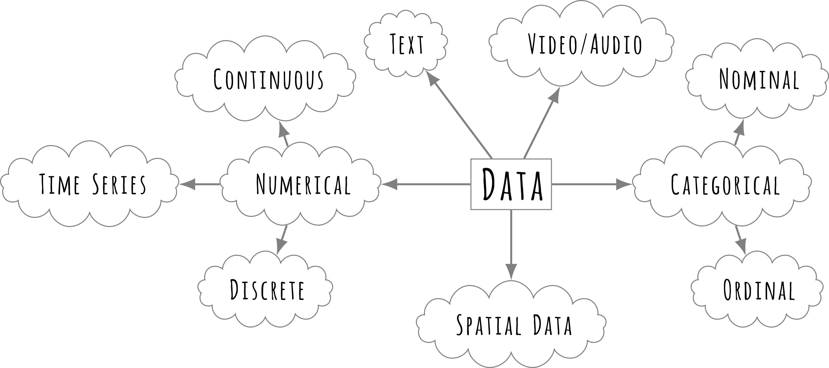
Another dimension for the classification of data is quantitative and qualitative. Within these, data can be further categorised based on its measurement level and characteristics.
Numerical, or quantitative data, consists of values that can be measured and expressed in numbers. It is used to perform mathematical computations and statistical analyses.
Discrete data represents countable values that take distinct, separate numbers, such as the number of students enrolled in a class, the number of questions answered correctly in a test, or the number of research papers published by a faculty member.
Continuous data, on the other hand, can take any value within a given range and is typically measured rather than counted. Examples include students’ heights and weights recorded in a physical education class, time taken by students to complete an on-line assessment, and the average marks obtained by students in an exam.
Categorical, or qualitative data, represents groups, labels, or classifications that do not have a numerical value but may be counted for frequency analysis.
Nominal data consists of categories that do not have a meaningful order or ranking, such as the different subjects chosen by students (e.g., Mathematics, Science, History), the types of schools (e.g., Government, Private, International), or students’ preferred learning styles (e.g., Visual, Auditory, Kinesthetic).
Ordinal data represents categories that have a meaningful order but do not have equal intervals between them. Examples include student performance ratings (such as Excellent, Good, Average, Poor), Likert scale responses in surveys (such as Strongly Agree, Agree, Neutral, Disagree, Strongly Disagree), and socio-economic status categories (such as Low, Middle, High).
Different types of data.
Another important data type in educational research is time-series data, which is collected at regular intervals to observe trends over time. Examples include the annual dropout rate in secondary schools over the past decade, monthly attendance rates in a school over a year, and the number of students enrolling in higher education institutions each year.
Additionally, spatial data includes geographical or locational information, such as mapping the distribution of literacy rates across different states, identifying regions with the highest school drop-out rates, and analysing school accessibility in rural and urban areas using Geographic Information Systems (GIS).
In recent times, biometric data has added another dimension to this list. Research studies often measure and analyse data that is derived from
In recent times, biometric data has added a sophisticated dimension to educational research. We can broadly classify this use into two categories:
1. Administrative Biometrics (Governance)
Research studies often measure and analyse data derived from digital identity systems to understand system efficiency. In India, this includes:
Attendance Monitoring: Using fingerprint or facial recognition data to track teacher and student presence, often to correlate attendance with academic performance.
Scheme Delivery: Analysing Aadhaar-linked data to study the reach of scholarships or Mid-Day Meals.
2. Cognitive Biometrics (Learning Science)
More recently, researchers are using physiological sensors to understand the process of learning itself.
Eye Tracking: By recording exactly where a student looks on a screen, researchers can study User Experience (UX) or reading patterns. For example, does a student focus on the diagram or the text when solving a physics problem?
Reaction Time & Stress: Measuring skin conductance or heart rate variability to assess “Exam Anxiety” or cognitive load during a complex task.
Unlike the static rows in a U-DISE spreadsheet, this type of data is high-frequency and complex. It often requires specialised R packages for analysis time-series data (e.g., thousands of eye-movement coordinates per minute).
Understanding the different types of data is crucial for selecting appropriate analysis methods and ensuring accurate interpretation of research findings. Choosing the correct type of data ensures that we as researchers can derive meaningful and reliable insights from the data.
Now that we have refreshed some of the basic ideas about data and its types let us look at some data using R.
Exercise
For each of the research questions discussed identify
The Independent Variable (IV) and the Dependent Variable (DV).
The Data Type for each (Nominal, Ordinal, Discrete, or Continuous).
3 Importing Data
To make statistical computations meaningful we will need data to work with. R has several excellent packages which provide data about various measurements. But to begin with we will see Along with these datasets in R, we will also see how to import data from external sources such as spreadsheets, csv files as these will be the ones we will work with.
We will start with a simple dataset, that of a classroom.
Suppose you are a teacher. You conducted tests in English, Science and Mathematics and have the following data of 30 students. Their name, roll number, age, gender, marks in three subjects (English, Science and Mathematics).
Roll No
Gender
English
Science
Mathematics
1
Male
88
92
84
2
Female
75
70
68
3
Male
65
60
72
4
Female
55
59
58
5
Male
45
49
51
6
Female
80
78
82
7
Male
42
47
40
8
Female
67
69
70
9
Male
85
87
89
10
Female
90
85
92
11
Male
33
38
36
12
Female
58
55
60
13
Male
60
62
63
14
Female
71
75
73
15
Male
48
45
42
16
Female
64
61
60
17
Male
50
48
46
18
Female
66
63
65
19
Male
38
44
41
20
Female
69
68
67
21
Male
77
79
80
22
Female
82
85
84
23
Male
43
47
45
24
Female
53
56
54
25
Male
91
93
95
26
Female
40
44
39
27
Male
87
89
86
28
Female
49
51
50
29
Male
46
42
48
30
Female
55
53
57
What does this table tell us at a glance? Not much, apart from telling the individual scores of the particular roll numbers. Typically such data are called as raw data. This data is arranged in a certain manner (by roll numbers) which does not tell us about the information we are concerned with. For example, consider the following questions:
What are the highest and lowest marks in each subject?
Which subject has the highest average? Which has the lowest?
How many students are scoring below the passing mark (35) in each subject?
What proportion of students are scoring between 35 and 50 (just passing)?
How many students scored 80 or above in at least one subject?
What is the distribution of total scores (English + Science + Mathematics), also by gender?
What are the average scores in each subject, also by gender?
What is the average mark in each subject (English, Science, Mathematics)?
What is the ranking of students according to these test results?
We will see how we can organise, transform and compute this raw data to give us answers to above questions.
For our purpose, this dataset is available as a CSV (Comma-Separated Values) file. CSV is a universal format for storing data in which each column is separated by a comma in every row, hence the name. Virtually all spreadsheet applications (like Excel or LibreOffice Calc) can open a CSV file.
Similar to CSV, you may encounter TSV (Tab-Separated Values) files. Beyond these text-based formats, we also have the common Microsoft Excel format (XLSX) and the open standard OpenDocument Spreadsheet (ODS).
R is capable of loading all these formats. In this section, we will focus on how to load our CSV file into R, as it is the most common format you will encounter in research.Note: All the datasets we will use are in the /data directory.
Loading A Data File in R
R has several dedicated functions to load datasets from files. For csv files we will use the read_csv function from the readr package. Let us see the syntax for loading the `csv` file.
# Load the tidyverse library (which includes readr for reading data)library(tidyverse)
── Attaching core tidyverse packages ──────────────────────── tidyverse 2.0.0 ──
✔ dplyr     1.1.4     ✔ readr     2.1.5
✔ forcats   1.0.0     ✔ stringr   1.5.1
✔ ggplot2   3.5.1     ✔ tibble    3.2.1
✔ lubridate 1.9.3     ✔ tidyr     1.3.1
✔ purrr     1.0.2
── Conflicts ────────────────────────────────────────── tidyverse_conflicts() ──
✖ dplyr::filter() masks stats::filter()
✖ dplyr::lag()    masks stats::lag()
ℹ Use the conflicted package (<http://conflicted.r-lib.org/>) to force all conflicts to become errors
# Read the data using read_csv (note the underscore _ )classroom_data <-read_csv("data/class-data.csv")
Rows: 30 Columns: 5
── Column specification ────────────────────────────────────────────────────────
Delimiter: ","
chr (1): Gender
dbl (4): Roll No, English, Science, Mathematics

ℹ Use `spec()` to retrieve the full column specification for this data.
ℹ Specify the column types or set `show_col_types = FALSE` to quiet this message.
Let us break down what this code does:
library(tidyverse): In the first line, we load the required package. If we do not do this, R will not know what read_csv means and will throw an error. Remember, you must load the library once per session.
read_csv("..."): In the second line, we call the function read_csv to read the file. Note the text inside the quotes: "data/class-data.csv". This is the file path. It tells R to look inside the data folder for a file named class-data.csv. If our file was in some other folder this file path would be different.
<- (The Assignment Operator): This arrow symbol is crucial and perhaps you would be using it more often than any other function in R. It tells R: “Read the file, and then save the result into an object named classroom_data.”
classroom_data: This is the name we chose for our data object. You could name it my_data or scores, but descriptive names are better. This object is stored as a dataframe (specifically, a tibble), which is the standard format for storing data tables in R.
3.1 An Interlude on File Naming and Organising
As a good researcher organising data in a meaningful way is a habit that you should develop. This includes how to name and organise your files and folders. Following are some best practices on how to give meaningful filenames in R (for R language and in general).
Do’s
Use descriptive, meaningful names.
-student_scores.csv, survey_data_2023.xlsx
Use only lowercase letters, numbers, hyphens (-), or underscores (_) instead of spaces.
Recommended: my_data.csv, class-01.csv
Avoid: My_Data.csv
Use consistent naming conventions.
For example:
Snake case: student_marks.csv
Kebab case: student-marks.csv
Include the correct file extension. Applications will not understand the type of file otherwise.
Use .csv, .xlsx, .R, .qmd, .txt, etc.
Don’ts
Do not use spaces in filenames. I cannot stress this enough. Avoid spaces in filenames to save yourself from lot of troubles later.
Do not use: student scores.csv
Preferred: student_scores.csv or student-scores.csv
Avoid special characters and punctuation. Some of these characters are reserved and can cause problems.
Do not use: ! @ # $ % ^ & * ( ) ~ ? > < ,
Do not start filenames with numbers, R does not like that.
Do not use: 2023_report.csv
Preferred: report_2023.csv
Do not hardcode absolute path
Do not use: read_csv("C:/Users/yourname/Documents/file.csv")
Use relative paths, as we have done in our example.
Do not rely on case-insensitivity
Data.csv and data.csv are treated differently, so be careful about letter cases in file names. It is best to use all lowercase letters to avoid any confusion.
3.2 Understanding the read_csv Output
When you run the read_csv code, R does not just silently load the file. It prints a message to the console that looks something like this:
Rows: 30 Columns: 5 ── Column specification ──────────────────────────────────────────────────────── Delimiter: "," chr (1): Gender dbl (4): Roll No, English, Science, Mathematics
Do not panic! This is not an error. It is a helpful status report. Let us decode it line by line:
Rows: 30 Columns: 5:
R is confirming that it successfully found 30 rows (students) and 5 columns (variables) in your file.
Check: Does this match what you expect? If you thought you had 50 students, something went wrong!
Delimiter: ",":
R correctly guessed that your file uses commas to separate values. (Some files use tabs or semicolons).
chr (1): Gender:
chr stands for Character (Text data).
R looked at the “Gender” column, saw letters like “Male” and “Female”, and decided to treat it as text.
dbl (4): Roll No, English...:
dbl stands for Double (Numeric data with decimals).
R looked at these four columns, saw numbers, and decided to treat them as numeric variables.
Why is this important?
Sometimes R guesses wrong. If you have a column for “Marks” but someone wrote “Absent” instead of a number, R might treat the whole column as chr (Text) instead of dbl (Number). This status report alerts you to such problems immediately.
At the end of the output, you will see two lines starting with the information symbol ℹ:
text
ℹ Use `spec()` to retrieve the full column specification for this data. ℹ Specify the column types or set `show_col_types = FALSE` to quiet this message.
These are helpful tips from R, not errors:
Use spec():
If your dataset has 100 columns, R won’t list them all in the console because it would be too long.
R is telling you: “If you want to see the detailed list of all 100 columns and their types (Text/Number), type spec(classroom_data).”
Quiet this message:
Once you are an expert, seeing this “status report” every time you load a file might get annoying.
R is telling you: “If you want me to load the file silently without printing this report, add show_col_types = FALSE to your command.”
For now, ignore these tips. As a beginner, seeing the column types is very useful to ensure your data loaded correctly.
3.3 “Seeing” the data in R
Now that we have added the data in R, how can we “see” this data?
4 Inbuilt datasets in R
Let us install some packages which provide several datasets. These are the learnbayes and MASS packages. To install them use the install.packages() function as shown below.
Load these two pacakges using the library() function.
Now within the LearnBayes and MASS pacakges we have several datasets. To see the datasets in a library we will use data() command. But using use data() will give all the datasets installed on your R system.
The following object is masked from 'package:dplyr':

    select
To see a datasets in a specific library we specify to data() that we want. For example the code block below will print the datasets in the LearnBayes package.
# view datasets in a particular library#data(package ="MASS")
This command will list all the datasets in the LearnBayes library. We will use some of the datasets to explore. We will use the dataset studentdata. To load this dataset we use data() command
# load the datasetdata("studentdata")data("survey")data("election")str(election)
Note how the str() command gives the variable names for each column and their class.
Which classes of datatypes can you identify in each set? Use the dim() function to find out the dimensions of the data. What do you expect the dimensions of the above dataset (they are tables after all)?
head() and tail()
The head() and tail() commands in R are used to quickly view the beginning and end of a dataset, respectively. These functions are particularly helpful when working with large dataframes or vectors, allowing users to inspect a small portion of the data without displaying the entire dataset.
head(): Displays the first 6 rows (by default) of a dataframe or vector. This is useful when you want to get a quick look at the structure or the first few entries of the data.
tail(): Displays the last 6 rows (by default) of a dataframe or vector. It’s useful for checking the most recent or final entries of your data.
tail(survey)
       Sex Wr.Hnd NW.Hnd W.Hnd   Fold Pulse  Clap Exer Smoke Height      M.I
232   Male   18.0   16.0 Right R on L    NA Right Some Never 180.34 Imperial
233 Female   18.0   18.0 Right L on R    85 Right Some Never 165.10 Imperial
234 Female   18.5   18.0 Right L on R    88 Right Some Never 160.00   Metric
235 Female   17.5   16.5 Right R on L    NA Right Some Never 170.00   Metric
236   Male   21.0   21.5 Right R on L    90 Right Some Never 183.00   Metric
237 Female   17.6   17.3 Right R on L    85 Right Freq Never 168.50   Metric
       Age
232 20.750
233 17.667
234 16.917
235 18.583
236 17.167
237 17.750
glimpse
The glimpse() function in R, provided by the dplyr package, offers a quick and concise overview of the structure of a dataframe or tibble. Unlike head() and tail(), which show only a subset of rows, glimpse() displays both the data types of each column and a preview of the data itself. This makes it especially useful for quickly understanding the composition and types of variables in a dataset.
glimpse(): Provides a transposed view of the dataframe, showing each column’s name, type, and a preview of its values. It helps to inspect the data structure in a compact form, particularly when dealing with wide datasets.
See Knuth (1984) for additional discussion of literate programming.