# Command to install R packages
# This is how you add comments in a code block
# Note that the package name is in double quotes

install.packages("rmarkdown")1 Introduction to Educational Research and R
1.1 Dramatis Personae
Curiosa: The central character of our story. She is a curious learner, and is full of all types of questions about all kind of things. She is our young researcher who has just set the journey towards doing educational research.
Simplicio: A peer of Curiosa (with apologies to Galileo) who is not curious and is likely to just get things done without understanding.
Faustus: A shady character who tries to derail the curious quest of Curiosa.
Pedagorgon: A classical pedagogue, doesn’t want any experiments in the classroom.
Also featuring at times in cameo roles:
Author: The opinions of the author. With this voice the author (mis)directs the thoughts of the reader and provokes them.
Reader: The opinions of the imagined reader. Though can also be called the B-team of the author.
2 What is research?
Research in any field provides its practitioners with a deeper understanding of fundamental aspects of the field. Likewise research in education intends to provides educators insights into various aspects of educational practice and theory. For example, a research study might investigate the effectiveness of a new teaching method on student scores, or how different teaching strategies affect the conceptual understanding in science. Learning about educational research requires both an understanding of research design and basic statistical concepts. In this book, we will touch upon the required ideas of research design, and dig deeper into the statistical ideas which substantiate them.

Any research is driven by questions, and framing good questions is equally important, perhaps more important, as the answers. Many scientific advances happened because certain questions were asked and answered. Framing a good research question is the first step towards research. Consider how the question ‘What is the structure of DNA?’ led to the discovery of the double helix, or ‘How do vaccines work?’ revolutionized public health. The research questions may arise from some gap in our understanding of natural world or some curiosity. For example, a researcher might ask ‘Does using mother tongue as the medium of instruction improve comprehension in early grades?’ We then seek to answer these questions by collecting data, and then analysing the data.
The type of research question asked will determine what research design we need to follow, what data we need to collect and how we analyse this data to answer our research question. Continuing the above example, one might collect assessment scores, interview the teachers, or carry out classroom observations from classrooms using different languages to answer our research question.
In educational research, we have two major types of data, namely, qualitative and quantitative. The type of analysis we perform depends on the nature of the data. In this book, we mostly deal with quantitative data. The data analysis then informs us about the questions we had raised, we may find correlations between variables, or causal relations between them, we may even form a theory. For example, analysing student scores in our mother tongue study we might find a correlation between use mother tongue in primary grades and higher scores. The answer to our question is shared with peers in the form of research reports, journals articles and presentations in conferences where it is put under scanner. This answer may raise further new questions and we are back to the first step. For example, analysing the mother tongue data might show a correlation with higher scores, but it might also reveal that teacher training with relevant language also matters. This leads to a new questions, new hypothesis, which required new data, and a new analysis. Thus research is often a cyclic process.
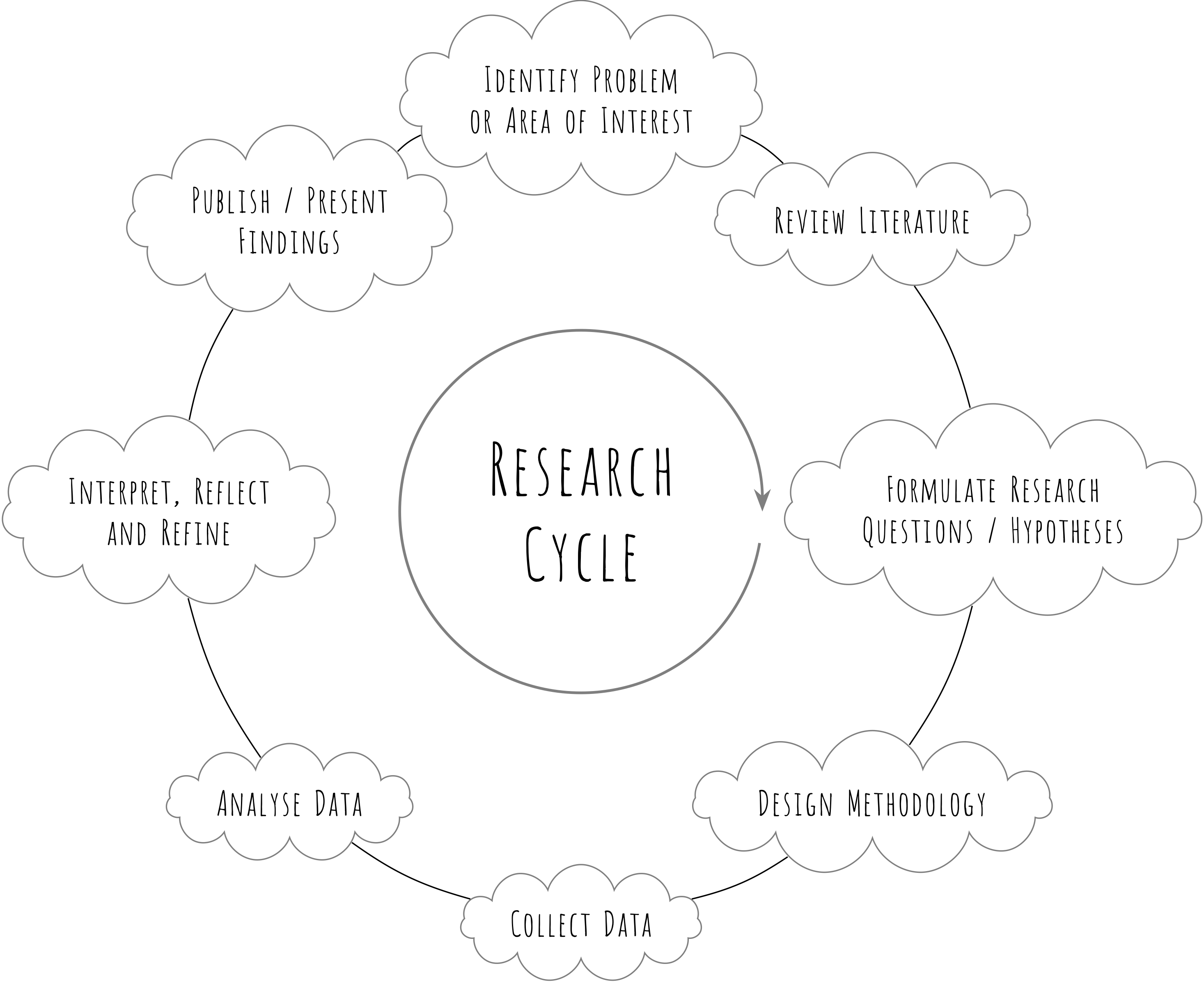
This process is sometimes called as the research cycle and involves continuous engagement between questions, assumptions, theory and data. While often seen as a practical manifestation of the scientific method, the research cycle applies more broadly to various forms of inquiry, not just experimental science. There are several steps, involved in the research cycle as shown in the broadly oversimplified figure above. Though not often stated explicitly, such a view also arises from and assumes specific philosophical views about the natural world. We briefly touch upon these views next.
In this work, we are assuming the position of realism, which holds a view that there is a reality independent of our perceptions. The understanding of this reality is always mediated by theories, perspectives and contexts in which we are working. Thus the research cycle is a cycle of approximation, aspiring for verisimilitude though never quite reaching it. Accordingly, all knowledge obtained through the research cycle is tentative knowledge that we can best assert to from the data that we have.
History of science is full of such examples where what was assumed to be true (by scientific consensus of the time) was later shown to be incorrect. Classic examples include the shift from the geocentric to the heliocentric model of the solar system, or the earlier belief in phlogiston theory before the understanding of oxidation. In context of education, the dominant theory of behaviourism was replaced by constructivist approaches starting from 1960s onwards. Thus, in realism the emphasis is on the the idea that knowledge evolves through successive cycles of observation, interpretation, and refinement. Thus in the case of our question about mother tongue we do not expect to find a final, unchangeable “Truth” that applies everywhere and forever. A significant result in our statistical analysis doesn’t mean we have “proven” the benefit of mother tongue once and for all. Rather, it means we have gathered strong evidence that approximates the reality of its benefits in our specific context. Future cycles of research might refine this knowledge, allowing us to have a more nuanced understanding of the issue. We are trying to build a model of reality that gets slightly more accurate, moving closer to the truth without ever claiming to strictly possess it.
Another assumption that is often found is that “data” are independent of theoretical framework and are bias free. But this assumption is not true. All data, even in so called hard-sciences, is “theory-laden” in the sense that theory brings context and meaning to the data. This means that theory determines not only how we interpret data, but even what we choose to collect as data in the first place. Without a theory, data has no context and cannot be understood.
Consider our example study on Mother Tongue instruction.
If we collect data purely on “Exam Scores” (Variable A), we are implicitly using a Behaviourist theory with the assumption that learning is best measured by output on a standardised test. However, if our theoretical framework is Constructivist, we might argue that only “Exam Scores” are insufficient data. We might instead choose to collect data on “Classroom Participation” or “Student Questions” (Variable B).
Both A and B are “data,” but our choice of which one to collect was driven by our theory of what “learning” actually is. Thus, the data itself carries the fingerprint of our theoretical beliefs.
In educational context, the cyclic view of research closely aligns with the philosophy of pragmatism as developed by John Dewey and Charles Sanders Peirce. Pragmatism treats inquiry as a problem-solving process, where ideas are tested and revised in practice. This inquiry is an iterative and reflective process informed by experience.
The knowledge inquiry generates is not static, it continuously evolves with new understandings and changing contexts. For example, early educational theories based on behaviourism often focused solely observable outcomes discounting any non-observable mental structures, but as our understanding of cognitive science evolved, more nuanced theories positing mental structures as being key to learning emerged. A good read on this is the book The Mind’s New Science: A History of the Cognitive Revolution by Howard Gardner.
Also inherent in both the positions above is the assumption that by studying the real (observing/experimenting) world we can understand it. This forms the basis of all our research. We will return to these issues several times later with context of interpreting our analysis of data, methodologies and inferring actionable outcomes.
Of course, we are over simplifying the philosophical accounts here, going any further will take us to deeper philosophical waters than we intend to go at this stage. But this philosophical background is often ignored because it is so “obvious” as this belief is rarely questioned. They often go in as assumptions which we take for granted. But being aware of these issues helps us engage better with research methods and their implications. A reminder that all research inquiry rests on particular ways of seeing and understanding the world and all our knowledge about the natural world is tentative and subject to change.
3 What type of questions can we ask?
3.1 Causality
One of the most important ideas in scientific research is trying to understand how two things are related. Research in general, and statistical methods in particular are used to establish if and how changes in one thing (A) are responsible for changes in another thing (B). Such a relationship is called as a causal relationship, and we say A causes B. For example, we believe (know?) that smoking causes lung cancer. But how did we come to this conclusion? What type of data and what analysis lead us to believe this causal connection?
In the physical sciences, establishing causality is often relatively straightforward. If you heat water in normal condictions to 100°C, it boils. Heat → Boiling.
But in education, causality is often messy.
Establishing a causal relationship is perhaps one of the most difficult tasks in educational research. Why? Because the “subjects” of educational research are complex entities and exist and interact with complex environments. It is often difficult to pinpoint exact “cause” of something that we observed.
Let us take an example. Imagine you find that private tuition (A) is related to higher math scores (B). Can you claim A causes B?
Maybe wealthy parents can afford both tuition and better nutrition/books. (This is a Confounding Variable).
Maybe students who are already good at math enjoy it more and ask for tuition. (This is Reverse Causality).
When we are certain that thing A causes thing B, we say that the relationship is causal. When we only know they move together, we say they are correlated.
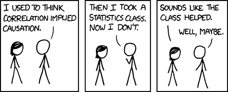
Golden Rule: Correlation does not imply Causation.
Just because schools with more libraries have better reading scores doesn’t mean building a library will automatically make a student a better reader.
This point, though reiterated often in statistics courses, is not understood well enough by many researchers. This cartoon by XKCD fame Rudolph Munroe hits the bullseye regarding this issue.
Quantitative educational research often follows a progression: it begins by describing the sample using descriptive statistics (like means and percentages), moves on to identifying patterns through correlations between variables, and finally employs rigorous research designs (such as Randomised Control Trials) to attempt to establish causation. The “progression” here refers to the hierarchy of evidence and complexity in quantitative research. It represents a journey from simply observing and summarising the data to understanding the mechanisms that drive it.
Of course not every research follows such progression. Many valuable studies are purely descriptive (for example, the Annual Status of Education Report, or U-DISE data), providing a snapshot of the current state of education without necessarily seeking to prove causal links. Other studies stop at the correlational level, identifying potential relationships that future researchers might investigate. The “right” stopping point depends entirely on the research question you asked at the beginning.
4 Types of Research Questions
Depending on their purpose, research questions can be classified into following types .
1. Descriptive Questions: The foundation
Questions answering “What is happening?”
Descriptive questions focus on summarising characteristics of data or phenomena without making predictions. They map the “lay of the land.” They answer “what,” “how,” “when,” and “where” questions using quantitative data (e.g., surveys) or qualitative observations.
Examples
- Infrastructure: “What is the current percentage of schools with functional girls’ toilets across all blocks in District X?” (Focus here is on magnitude and distribution).
- Enrollment: “What is the Gross Enrollment Ratio (GER) for Scheduled Tribe (ST) students in secondary schools over the last five years?”
2. Exploratory Questions: The Search for Patterns
Questions Answering: What is the hidden pattern?
Exploratory questions aim to investigate unknown or poorly understood phenomena. They are open-ended and flexible, focusing on generating new insights, ideas, or hypotheses rather than definitive answers.
Use Cases
Dropout Analysis: “Is there a correlation between the month of the year and student dropout rates in agricultural districts?” (Looking for harvest-season patterns).
Resource Utilization: “Is the under-utilization of school libraries associated with the distance of the library from the main classroom block, or simply the lack of a dedicated librarian?”
3. Inferential Questions: The Connection
Questions Answering: Is X related to Y in the population?
Inferential questions seek to draw conclusions about a population based on sample data. These questions often involve statistical inference techniques, such as regression analysis, correlation studies, or hypothesis testing. They aim to uncover relationships, predict outcomes, or generalise findings.
Examples
Prediction: “How does parental income influence the likelihood of a student completing Class 12?” (Generalizing from a sample survey to the state population).
Teacher Qualifications: “Is there a significant relationship between teacher experience (in years) and student math achievement across the state?”
4. Confirmatory Questions: The Test
Questions Answering: Is our theory/model correct?
Confirmatory questions are designed to test specific hypotheses or predictions. They aim to validate or refute pre-existing theories or assumptions using empirical data. These questions are typically used in quantitative research and rely on statistical methods to determine relationships, effects, or differences.
Use Cases
Intervention Testing: Hypothesis: “Does the new ‘Math-Lab’ intervention lead to a statistically significant increase in geometry scores compared to the traditional method?”
Policy Impact: Hypothesis: “Did the introduction of the Mid-Day Meal scheme successfully reduce the ‘Gender Gap’ in attendance by more than 10%?”
Sometimes we group Inferential, Confirmatory questions under the label ‘Analytical Research’, as they go beyond mere description to analyse the underlying relationships between variables.

| Type | Category | Description | Example (Educational Context) |
|---|---|---|---|
| Qualitative | Exploratory | Seeks to understand perspectives and meanings without influencing results. | “What are teachers’ initial thoughts on the new National Education Policy?” |
| Qualitative | Interpretive | Examines individuals’ behaviour and cultural meaning in natural settings. | “How do university researchers perceive AI’s role in academic publishing?” |
| Qualitative | Experiential | Focuses on understanding individuals’ lived experiences and perspectives. | “What are the challenges rural students face during their transition to urban colleges?” |
| Quantitative | Descriptive | Measures responses of a population regarding a particular question or variable. | “How often do Grade 10 students use online learning platforms?” |
| Quantitative | Exploratory (EDA) | Uses statistical and visual methods to summarise dataset characteristics. | “What patterns can be observed in state-wide dropout rates over the last decade?” |
| Quantitative | Comparative | Investigates differences between two or more groups regarding an outcome. | “How do math scores differ between students in Government vs. Private schools?” |
| Quantitative | Correlational | Examines relationships between two or more variables without implying causation. | “What is the relationship between teacher salary and job satisfaction?” |
| Quantitative | Predictive | Uses statistical models to estimate future trends or outcomes. | “Can student attendance in the first month predict their final exam grades?” |
4.1 Research Methods
In research a distinction is made between qualitative and quantitative research methods. Sometimes the design incorporates both types of methods known as the mixed method. This distinction is primarily because of the type of data that is collected, and the methods used for analysis of the data. In this book, we will primarily look at the quantitative aspects of data analysis.
Many methods of quantitative analysis of data which are statistical in nature were developed in the last hundred years. Qualitative methods are more recent in origin. Another aspect of the data analysis which has really prospered in recent times is improvement in data visualisation methods. R has excellent libraries for both aspects. We will look at various concepts statistical analysis using R, i.e. all computations will be made using R and in the process introduce the syntax, functions and libraries of R.
Exercise
Create at least two research questions of each of the four categories listed above.
For each question, complete the following structure:
The Question: (Does teacher training affect student scores?)
The Rationale: Why is this question worth asking? Who will benefit from the answer? (Policymakers need to know if the training budget is well spent.)
The Data Required: Be specific. What variables would you need to measure? (I need ‘Teacher Training Hours’ and ‘Student Math Scores’ from 50 schools.)
I am assuming a basic familiarity with some basic statistical concepts. But in any case we will try to be thorough with the conceptual understanding of the topic at hand and its applications.
I will try to provide historical context for the development of these ideas when possible. We will use some of the inbuilt datasets in R for discussion some concepts and some datasets that were derived from various sources.
5 What is R?
R is a programming language for statistical computing, data analysis and graphics. R widely used in data analysis, statistics, and machine learning in both academic and industry. R is particularly powerful for data visualisation and statistical modelling. R is highly extensible due a vast ecosystem of packages/libraries (over 18,000 on CRAN) for specialised tasks, so if there is a need for a particular task chances are that there is already a library for it. Finally R is cross-platform, it runs on Windows, macOS, and Linux, making it accessible to users on any operating system. Added advantage is that same programme will run across computers.
R was developed in the early 1990s by Ross Ihaka and Robert Gentleman at the University of Auckland, New Zealand. It was inspired by the S programming language developed at Bell Labs in the 1970s. R was officially released as Free Software under the GNU General Public License (GPL) in 1995. Because R is Free Software, the users don’t have to pay for its use or distribution. Being Free Software it also allows you to use it for any purpose, view the source code, modify and source code and distribute it to anyone with similar license. Thus you can share R with to your colleagues, friends and family members without any issues and have a legal right and moral responsibility to do so.
Growth and Popularity
The Comprehensive R Archive Network (CRAN) was established in 1997 to distribute R packages. R gained popularity in data science, statistics, and academia due to its flexibility and vast package ecosystem. Today, R is used by millions of statisticians, data scientists, and researchers worldwide. Major corporations, now use R for data analysis.
Tidyverse Revolution: In the 2010s, Hadley Wickham and colleagues developed the tidyverse, a collection of R packages for data science
RStudio: The development of RStudio (now Posit) in 2011 made R more accessible with a user-friendly development environment. We will use R Studio in this book. R Studio is released under AGPL 3.
A large community of R users in various fora, resources and tutorials exists which makes getting help easy.
5.1 Why Use/Learn R?
Flexible scripting capabilities for automation and reproducibility. R can also use data from many sources and formats such as csv, xlsx, spss etc. R also provides support for mathematical typesetting using LaTeX. R Studio also provides us with options to create full reports, books, presentations and interactive visualisations and dashboards. It is also possible to export them to various formats like HTML, EPUB, PDF and DOCX or even create websites. This book was itself written in R Studio using the bookdown library of R.
5.2 Some Examples of R
- R Galleries
- Interactive Visualisations/Widgets using Shiny
- GGPLOT2 Extensions
5.3 Installing R and RStudio
To start using R via R studio, you will need to first install R and then R Studio. Please remember the order of installation. The RStudio Website provides links for both installations.
Difference Between R and RStudio
For new users there is often a confusion between R and RStudio the image below from R Coding for Data Science by Michela Cameletti is a good example of that difference.
The RStudio setup once done by default looks something like below. It may look intimidating and confusing first, but we will get used to it.
5.4 First Steps in R
At the first glance the R Studio interface looks a bit intimidating. There seem to be too many options with no clear indication of how to use it. Don’t worry, we will start using some basic commands. I will highly recommend use of R Markdown (RMD) or equivalently Quatro Markdown (QMD) format for using R Studio. With QMD (or RMD) format you can write text and code in the same file and see the results of the code (such as numbers, tables or graphs) in the final output.
You can refer to the R Studio cheatsheet here to get a basic orientation of the interface.
The R Studio interface has four panes. The basic idea of programming with R Studio is that you write the code in the upper left corner window (the editor) and its output will be see in the lower left terminal, or in the lower right window.
The windows and their placement is configurable in the Seetings.
Markdown Format
Markdown is a simple document format which allows us to write structured documents using simple text. For example, to create a section in the document we use the # for a subsection we use ## etc. Table Table 5.1 shows some basic commands of the markdown format.
| Feature | Markdown Syntax |
|---|---|
| Heading 1 | # Heading 1 |
| Heading 2 | ## Heading 2 |
| Heading 3 | ### Heading 3 |
| Bold | **Bold Text** |
| Italic | *Italic Text* |
| Bold + Italic | ***Bold Italic*** |
| Unordered List | - Item 1 - Item 2 |
| Ordered List | 1. First 2. Second |
| Inline Code | `code` |
| Code Block (R) | ```{r} plot(1:10) ``` |
| Blockquote | > Quoted text |
| Links | [Text](https://example.com) |
| Images |  |
| Tables | | Col1 | Col2 | |------|------| | Data | Data | |
The reason I am introducing this first so that you can create documents in R Studio which you will work on as we progress through the book.
You can see this excellent primer on using R Studio and R Markdown format.
Some more useful commands in RMD format are given in the cheatsheet.
5.5 Base R functions
Some functions in R known as base-R functions which are always available when you start R. They provide essential tools for data manipulation, statistical analysis, and visualization. For example, basic arithmetic operators like + - * \ are always available. Also some of the plotting functions like plot() and some statistical/mathematical functions like mean(), sum() are always available. For more extended functionality, R has different packages which provide specific functions.
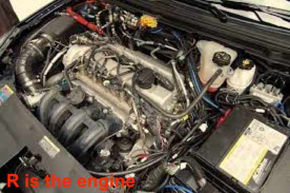
Another way to look at this is that base-R functions are like a basic car model. To get the additional functionality we need to get other things installed on this base model of the car. Similarly, in R we need to install libraries to get additional functions.
Code Blocks
We type commands in R at the window known as the console. You will have the > as prompt. All the messages pertaining to the command execution, including the error messages, will appear here. If the output of the command is a graphic, it will appear in the Viewer window on right hand lower side. Similarly any data sets and their summaries will appear in the Environment window (right hand top side).
You can insert codes in a markdown file which can run the code and display its output. For example, the code block below shows how to install packages in R.
Do not forget to add the quotation marks around the package name. Also note that R Studio has an auto-complete feature so that it can help you write the code as well. Now you know how to install new packages in R! We will install other packages as required. To get help on any package you can click and search in the Help window in the Viewer part of R Studio. If you do not add quotes the command will throw an error. It is essential to also understand the errors that we get when R syntax is not correct.
Using R Studio and R markdown (RMD) format we typically write our code in special sections in the RMD file. These sections are called as “chunks”. There are “text chunks” (like this one) and “code chunks” like what we have see. A code chunk allows you to write and execute R code inside the Markdown document. You can name the chunk, set options for evaluation, control what gets displayed, and much more. Below is a simple example with the expression 5 + 3, where we will see different aspects of the R code chunk.
Let us look at some simple variations on how this simple example will give different outputs in the rmd file depending on the options that we give to the code chunk.
The code chunk will start and end with three quotes “```”. After this you need to specify the language we are using for this chunk in our case “r”, and name of the chunk. There are other options which we explore below.
Code Chunk Variations
This chunk will be visible and will be evaluated. The result will be given in the output.
5 + 11[1] 16This chunk will not be evaluated
5 + 3This chunk will be evaluated, but code will not be displayed
[1] 8See the corresponding output in the HTML file.
Exercise
Try these commands and see if the output is correct.
5*85^85.6 Tidyverse
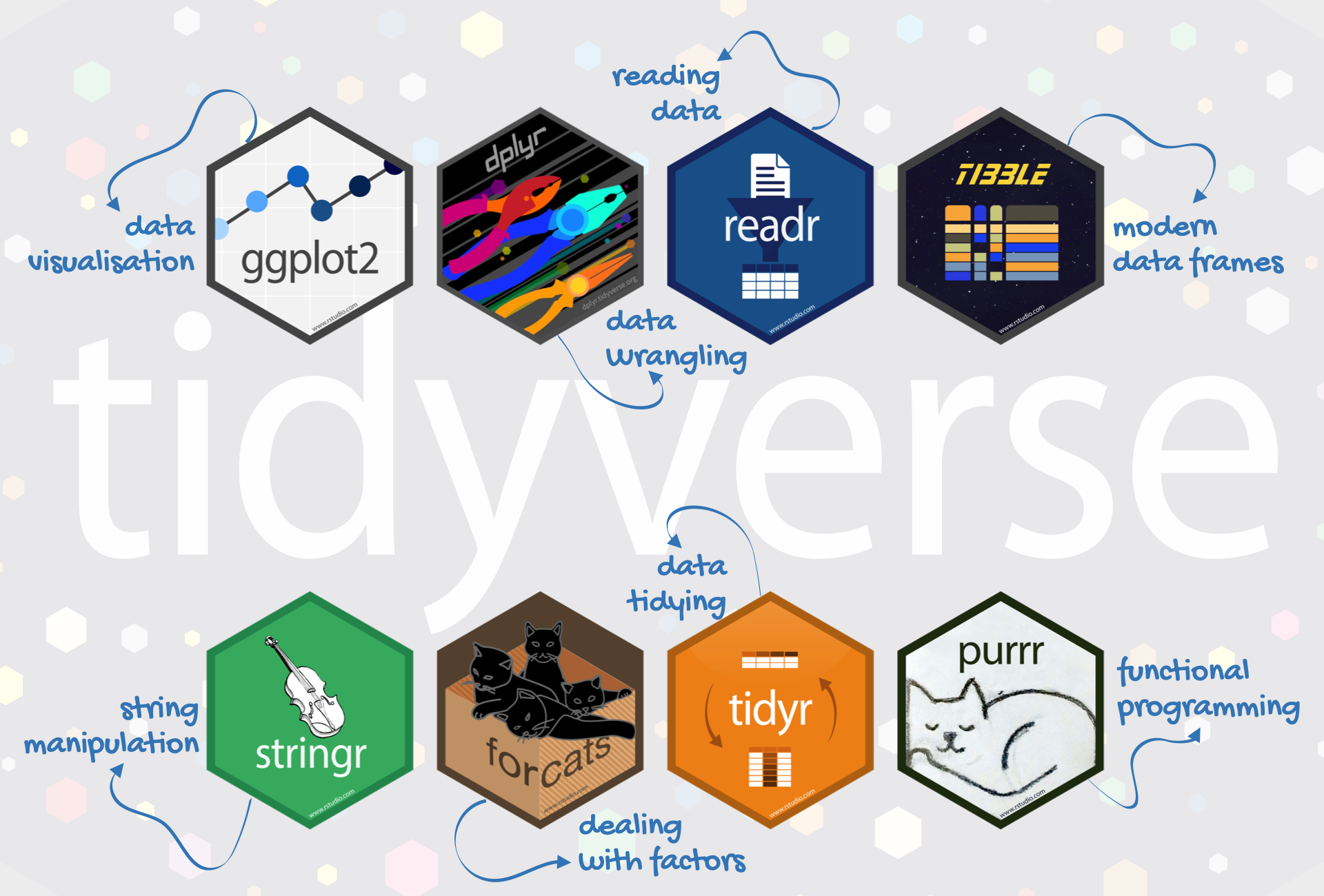
One of the most powerful packages in R is the tidyverse package. Tidyverse is actually a collection of eight packages. We will get several packages with tidyverse including very powerful ggplot2 and dplyr packages. If any other packages are required we will install them later.
Install the tidyverse package using the command above.
You can have a look at the various components of the tidyverse here.
After installing the package you will need to “load” the package to the current working space. Without loading the package to the current working space you cannot use it. The syntax to load a package is as follows:
library("rmarkdown")
library("tidyverse")
Exercise
Load the tidyverse, package using the above command. If you have not installed tidyverse you will get an error.
At this point I want to clarify a confusion that I have often seen about installing packages and loading them. You have to install the packages only once on your system (this is done using the install.package() command. When you close R Studio the packages will remain installed, you do not need to install them again. But each time you restart R Studio you will need to load the packages using library()each time so that they are accessible to you. If you do not load the packages the commands of that package will not be accessible to you and you will get errors while running those commands. We will see some examples of the typical errors when we start coding.
In the next chapter we will look at what is data, its types and how to import and “see” data in R.