Descriptive statistics is the term used when we are trying to describe the data in a meaningful way. This usually means presenting the data in a summarised or a visual-graphical form. Let us clarify what we mean by this with an example.
Suppose you are a teacher. You conducted tests in English, Science and Mathematics and have the following data of 30 students. Their name, roll number, age, gender, marks in three subjects (English, Science and Mathematics).
Roll No
Gender
English
Science
Mathematics
1
Male
88
92
84
2
Female
75
70
68
3
Male
65
60
72
4
Female
55
59
58
5
Male
45
49
51
6
Female
80
78
82
7
Male
42
47
40
8
Female
67
69
70
9
Male
85
87
89
10
Female
90
85
92
11
Male
33
38
36
12
Female
58
55
60
13
Male
60
62
63
14
Female
71
75
73
15
Male
48
45
42
16
Female
64
61
60
17
Male
50
48
46
18
Female
66
63
65
19
Male
38
44
41
20
Female
69
68
67
21
Male
77
79
80
22
Female
82
85
84
23
Male
43
47
45
24
Female
53
56
54
25
Male
91
93
95
26
Female
40
44
39
27
Male
87
89
86
28
Female
49
51
50
29
Male
46
42
48
30
Female
55
53
57
What does this table tell us at a glance? Not much, apart from telling the individual scores of the particular roll numbers. Typically such data are called as raw data. This data is arranged in a certain manner (by roll numbers) which does not tell us about the information we are concerned with. For example, consider the following questions:
What are the highest and lowest marks in each subject?
Which subject has the highest average? Which has the lowest?
How many students are scoring below the passing mark (35) in each subject?
What proportion of students are scoring between 35 and 50 (just passing)?
How many students scored 80 or above in at least one subject?
What is the distribution of total scores (English + Science + Mathematics), also by gender?
What are the average scores in each subject, also by gender?
What is the average mark in each subject (English, Science, Mathematics)?
What is the ranking of students according to these test results?
We will see how we can organise, transform and compute this raw data to give us answers to above questions.
Some of these questions can be answered by sorting data in a different way. Right now it is being sorted by a label, the roll number, which doesn’t have any inherent meaning, it is neither ordinal or nominal. Well in some cases the roll number maybe based on alphabetical names, or order in which students were admitted to the class, but for our present case, it is just an identifier of the student.
Some questions can be answered by sortingand taking counts below or above a particular threshold (marks = 35, marks = 80 etc.). In remaining questions we need to take means of the data. Still further we need to group the data and then take the means.
⁉️ Identify which questions can be answered how? {#sec-⁉️-identify-which-questions-can-be-answered-how}
Let us load this data in R. We will use the csv (comma-separated value) file. To load this file you can use this command
This command will import the data into R and store it in an object called classroom_data. Let us understand what each line and command does. The first line library(here) uses a R package called here which allows relative paths to be given. The package constructs file paths relative to the project root (usually where your .Rproj file or Quarto project root is present. This way problems of working in different directories is sorted. (Your computer folder structure will not be same as mine.) More on this later.
To actually read the csv file we use the function read.csv(...) which is a base R function, that means it comes with default installation of R and you do not need any library to be installed to use it. Then the actual folders and files: "data" is the name of the folder and "class-01.csv" is the name of the CSV file inside this folder. Finally class.data <- ... stores the result of reading the CSV file into an object called classroom_data.
Now that we have our data loaded in R as classroom_data let us see this data. To see the data in R we simply type the object name.
Now the object containing our data classroom_data is stored in a particular manner. It has the class as data.frame. You can check this using the command class(...).
Rows: 30 Columns: 5
── Column specification ────────────────────────────────────────────────────────
Delimiter: ","
chr (1): Gender
dbl (4): Roll No, English, Science, Mathematics

ℹ Use `spec()` to retrieve the full column specification for this data.
ℹ Specify the column types or set `show_col_types = FALSE` to quiet this message.
# class(classroom_data)
In R, a dataframe is a fundamental data structure used to store data as a table, just like a spreadsheet. Each column in a dataframe can hold values of different type of variables such as numbers, text, or categories and each row represents an observation or record. Note that in a dataframe all columns must contain the same number of rows.
There are various functions that are useful to access, manipulate and transform the datatable. We will see some of them now.
Now each column of the dataframe can have different data types. For example the first column is the Roll number, let us check its data type. For this we will need to tell the class(...) function that we only want to know the data type of the first column. There are two basic ways of doing this. Both can be useful depending on the situation.
Case 1: By column name
In this case we specify the column name of the dataframe. For example,
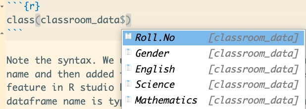
class(classroom_data$Roll.No)
Warning: Unknown or uninitialised column: `Roll.No`.
[1] "NULL"
Note the syntax. We used a $ sign after the dataframe name and then added the column name. The autocomplete feature in R studio helps a lot in this. Once the dataframe name is typed and $ added, it will show all the column names as shown below.
Autocomplete feature in R studio.
You can just select the required column.
Case 2: By column number
In this case we specify the column number of the dataframe. There are multiple ways to achieve this
class(classroom_data[[1]])
[1] "numeric"
#returns the first column as a vectorclass(classroom_data[, 1])
[1] "tbl_df" "tbl" "data.frame"
#same as above, returns the first column
Note that we use [[...]] two square brackets to specify the column. In the second case, [, 1] we are selecting the first column. This format can also be used to select rows or specific cells. The table below shows how we can access different elements of the dataframe by this format.
Syntax
Meaning
Returns
df[i, j]
i-th row and j-th column
A single value, the i-j-th cell.
df[i, ]
i-th row, all columns
A row (as a data frame)
df[, j]
all rows, j-th column
A column (vector or data frame)
df[, 2:5]
all rows, columns 2 to 5
A sub-data-frame
df[[j]]
j-th column
A vector (drops dimensions)
df[, "name"]
column by name
Same as df[[j]] if exact match
The commands in the table above can be used in a variety of ways to extract required data, either as columns or as sub-datasets. For example, if we only want a table that has roll number and science scores we can again use the column names or column numbers.
Let us check the output of this command which takes out values of Roll.No (Column 1) and science scores (Column 4).
What we have done here is to create a vector using the “combine” or “concatenate” function c(...) . This function will create a vector with entries that we have given, namely 1 and 4. Thus our command [, c(1,4)] will give us
All rows (because nothing is specified before the comma),
Only columns 1 and 4 (because c(1, 4) selects these two columns by position).
We can use similar syntax `c(...)` to get very specific data out of a dataframe.We can also use column/row names instead of numbers. In this the name string has to be inside quotes "name".
Note we cannot write [,1,4] it will give an unexpected answer.
Task
Use column names instead of column numbers to get the same subset of two columns.
But note that there are a total of three columns two columns of roll number and one for Science. This is clearly wrong. We had asked only for 2 columns! What is happening? The thing is that R adds row numbers also while displaying the data in this case. Notice that there is no column name in the first column. This feature is useful at times. But if we do not want this row numbers we can suppress this using
Enough of R commands, let us do some statistics on the data set. At the beginning we asked some questions about the classroom data.
Let us start with the first one
What are the highest and lowest marks in each subject?
For this we have two dedicated functions in R min(...) and max(...) to find out minimum and maximum values in a given data. The syntax is min(x) where x is set of the data values. In our case for each subject, we have column names. These can be seen with the command names(...):
Thus, to get maximum values of English scores we can write
max(classroom_data$English)
[1] 91
Similarly, for minimum value we can write
min(classroom_data$English)
[1] 33
Task
Find out minimum and maximum values of Science and Mathematics scores. For science scores use the column name method, and for mathematics use column number method.
We can also save the output of the commands like min(...) to a specific variable. For example, let us store the minimum and maximum scores in English with variables eng_min and eng_max
Note that the above code block does not produce any results. This is because we have only computed and stored the minimum and maximum values to the variables eng_min and eng_max. To see these values we can just type the variable names.
eng_min
[1] 33
eng_max
[1] 91
Task
Store min and max values of Science and Mathematics scores in suitably named variables.
Now let us see how we can present the results in a nice table using package called as knitr(...). For this we will use slightly different approach
library(tidyverse)
── Attaching core tidyverse packages ──────────────────────── tidyverse 2.0.0 ──
✔ dplyr     1.1.4     ✔ purrr     1.0.2
✔ forcats   1.0.0     ✔ stringr   1.5.1
✔ ggplot2   3.5.1     ✔ tibble    3.2.1
✔ lubridate 1.9.3     ✔ tidyr     1.3.1
── Conflicts ────────────────────────────────────────── tidyverse_conflicts() ──
✖ dplyr::filter() masks stats::filter()
✖ dplyr::lag()    masks stats::lag()
ℹ Use the conflicted package (<http://conflicted.r-lib.org/>) to force all conflicts to become errors
Here we have used one of the most powerful functions in R. The summarise(...) function, also works with summarize(...) in American English. It is used create summary statistics from a data frame. summarise(...) collapses multiple values into a single summary value. In our case we are applying it to a column in a dataframe.
Also we have added another function mean(...) to the set, this gives us the mean value of the set (in this case the science scores). The mean(...) function gives 5 decimal points in the computation. We need to round this to 2 decimals. For this we can use the round(...) function. The round(x, digits = n) function takes two arguments, first the numeric object x to be rounded and second, the number of decimal places needed n. The default number of decimal places to round to is 0. For example, `round(3.14159, digits = 2)` gives us 3.14.
To create a summary table for all subjects, the code can be like as follows:
We can make this block of computations more efficient by using loops. Suppose you have 30 columns in your table, you are certainly not going to write each individual column name. The same table can be computed as under
summary_all <- classroom_data |>summarise(across(.cols =c(Science, English, Mathematics),.fns =list(Min = min,Max = max,Mean =~round(mean(.x), 2) # rounding here ),.names ="{.col}_{.fn}" )) |>pivot_longer(everything(),names_to =c("Subject", ".value"),names_sep ="_")knitr::kable(summary_all, caption ="Scores Summary for All Subjects")
Scores Summary for All Subjects
Subject
Min
Max
Mean
Science
38
93
63.13
English
33
91
62.40
Mathematics
36
95
63.23
Let us understand this across() applies min, max, and mean to the selected columns (Science, English, Mathematics)
.names = "{.col}_{.fn} ensures consistent naming for pivot_longer to separate by _
pivot_longer() then reshapes it to a tidy format for your table.
The pivot_longer() function from the tidyr package is used to transform data from wide format to long format. It collapses multiple columns into key-value pairs, which is especially useful for tidy data principles, where each variable should have its own column and each observation its own row. The syntax is as follows pivot_longer(data, cols, names_to, values_to). Here
data: the data frame.
cols: columns to be collapsed.
names_to: name of the new column that will hold the former column names.
values_to: name of the column that will hold the values.
Another useful function is the summary(...) function. This function gives a statistical summary of different columns in a dataframe. The type of summary depends on the datatype of the column. For example, to get summary of classroom_data we can use
summary(classroom_data)
    Roll No         Gender             English         Science
 Min.   : 1.00   Length:30          Min.   :33.00   Min.   :38.00
 1st Qu.: 8.25   Class :character   1st Qu.:48.25   1st Qu.:48.25
 Median :15.50   Mode  :character   Median :62.00   Median :60.50
 Mean   :15.50                      Mean   :62.40   Mean   :63.13
 3rd Qu.:22.75                      3rd Qu.:76.50   3rd Qu.:77.25
 Max.   :30.00                      Max.   :91.00   Max.   :93.00
  Mathematics
 Min.   :36.00
 1st Qu.:48.50
 Median :61.50
 Mean   :63.23
 3rd Qu.:78.25
 Max.   :95.00
This statistical summary has the minimum, median, mean, maximum and first and third quantiles for numerical data. For text data it gives length of the column (30) and type of data. Check this summary against the data that we have calculated earlier.
We can also use the computations or objects right in the text. For example, we can call the mean the mean score of science that we have computed earlier, in this sentence. To use the inline R values we simple put them in quotes like this (this quote is the left of “1” of your keboard).
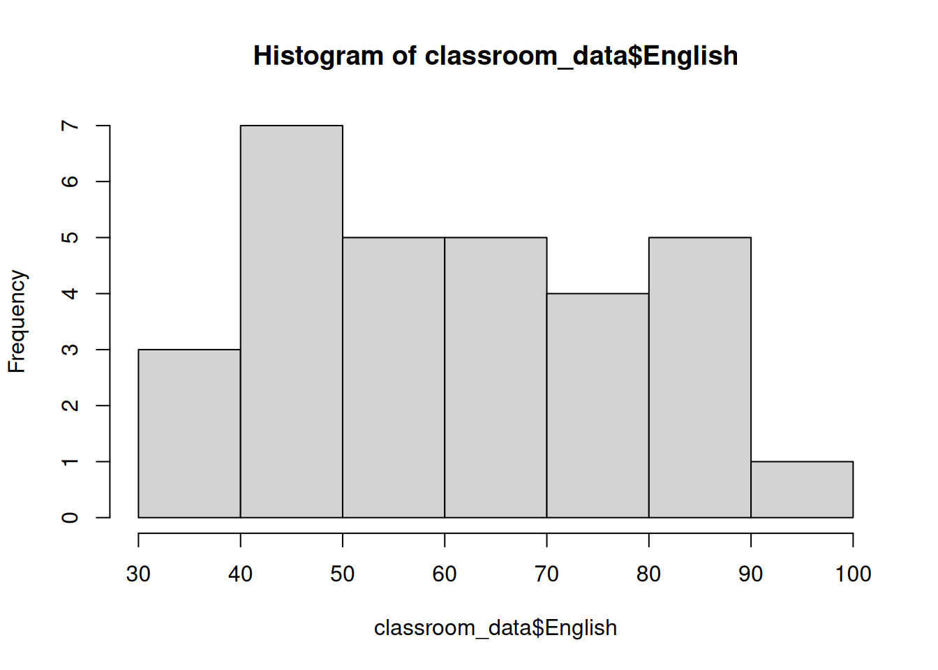
hist(classroom_data$English)
6 One Variable Analysis
6.1 Frequency distributions
6.2 Central Tendencies
Central Tendency and Variability
Measures of Center
Mode: mode, crude mode, and refined mode.
Median: median, rough median, and exact median.
Mean: mean, grouped mean, weighted mean, pooled mean, and mean of dichotomous variable.
Other order measures: midextreme (midrange), midhinge, trimean, and biweight.
Other means: trimmed mean, winsorized mean, and midmean; geometric mean, harmonic mean, generalized mean, and quadratic mean.
Measures of Spread
Numeric: mean deviation (average deviation), population variance, population standard deviation, sample variance, sample standard deviation, pooled variance, variance of dichotomous variable, coefficient of variation (coefficient of relative variation), and Gini’s mean difference.
Ordinal: range, interquartile range (midspread), quartile deviation (semi-interquartile range, quartile range), coefficient of quartile variation, median absolute deviation, coefficient of dispersion, and Leik’s D. Nominal: variation ratio, index of diversity, index of qualitative variation, entropy, and standardized entropy.
Sampling distributions: variance of sampling distribution of means, standard error of the mean (standard deviation of sampling distribution of means), standard error of a proportion, and sampling error.
6.3 Summaries: Tabular and Graphical
Statistical Graphics for Univariate and Bivariate Data
Statistical Graphics for Visualizing Multivariate Data
# Relating Statistics and Experimental Design : An Introduction
Methods of Randomization in Experimental Design
6.4 Spread
6.5 Tables
6.6 Graphs
6.7 Normal and abnormal?
7 Two or more Variables
7.1 Tables
8 Inferential Statistics
8.1 Reliability and validity
Research Designs
Introduction to Survey Sampling
Achievement Testing: Recent Advances
Using Published Data: Errors and Remedies
Secondary Analysis of Survey Data
Bayesian Statistical Inference
Cluster Analysis
Models for Innovation Diffusion
Meta-Analysis: Quantitative Methods for Research Synthesis